前面我们已经了解神经网络的各个组成部分,以及一些基本的层,比如全连接层,ReLU层等,现在是时候开始搭建一个简单的神经网络了!
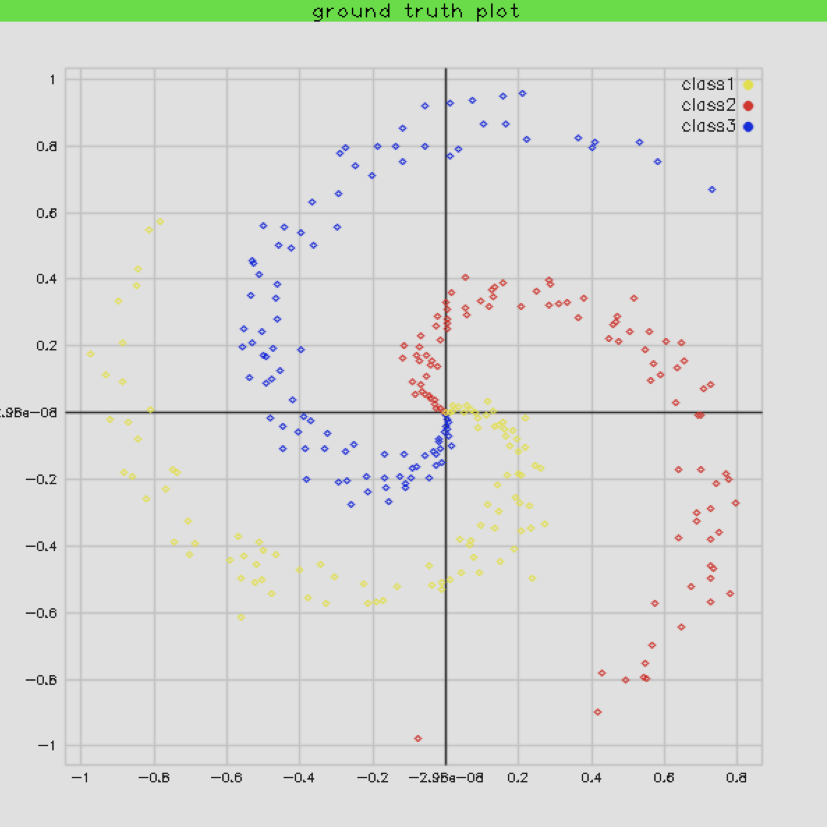
我们的目标是训练一个神经网络来对二维平面上的点进行分类。
训练数据准备 首先让我们生成一些训练数据,这些训练数据总共有3类,每类100个点,每个点的维度是2(即x,y坐标)。为了把数据作为 caffe2 的网络输入,比较合适的方法是把数据写入到 leveldb 中去,然后使用操作数据库的操作子去读取。生成及写入数据库的代码这里就不赘述,可以参考代码仓库 。
这些点在平面上的分布是这样的:
创建神经网络 生成了训练数据库后,可以使用caffe2_cpp_tutoria中的ModelUtil帮助类去创建网络,首先我们尝试看看线性网络能不能正确地把这三类点分开,下面就是我继承这个类设计的一个线性网络(只有一个直连层):
1
2
3
4
5
6
7
8
9
10
11
12
13
14
15
16
17
18
19
20
21
22
23
24
25
26
class FCModel : public ModelUtil { public : FCModel (NetDef &initnet, NetDef &predictnet) : ModelUtil (initnet, predictnet) {} OperatorDef *AddFcOps (const std::string &input, const std::string &output, int in_size, int out_size, bool relu = false ) init.AddXavierFillOp ({out_size, in_size}, output + "_w" ); predict.AddInput (output + "_w" ); init.AddConstantFillOp ({out_size}, output + "_b" ); predict.AddInput (output + "_b" ); auto op = predict.AddFcOp (input, output + "_w" , output + "_b" , output); if (!relu) return op; return predict.AddReluOp (output, output); } std::string Add (const std::string input_name, int in_size, int out_size) { predict.SetName ("FC" ); predict.AddInput (input_name); std::string layer = AddFcOps (input_name, "fc1" , in_size, out_size, false )->output (0 ); layer = predict.AddSoftmaxOp (layer, "prob" )->output (0 ); predict.AddOutput (layer); return layer; } };
在实际使用这个类的时候,如果需要训练,那么要对这个网络前面加上数据输入层,以及在后面加上loss层:
1
2
3
4
5
6
7
8
9
10
void create_net (FCModel& fc_model, bool deploy = false ) if (!deploy) { fc_model.AddDatabaseOps ("db" , "data" , db_path, db_type, K * N); } std::string output_layer = fc_model.Add ("data" , D, K); if (!deploy) { fc_model.AddTrainOps (output_layer, lr, optimizer, stepsize, gramma); } std::cout << fc_model.Short () << std::endl; }
训练 实际训练用的最多的是 sgd 算法,通常会确定一个初始的Learning rate(这里我设置的是0.1),然后每个iter中让这个初始学习率乘以一个系数,这个系数可以通过stepsize 和 gramma 这两个参数算出:
1
2
3
4
5
6
7
8
9
10
11
12
13
14
15
16
17
18
19
20
21
22
23
24
25
26
27
28
29
30
std::string optimizer = "sgd" ; const double lr = 1 ;const int stepsize = 10 ;const float gramma = 0.999 ;const int iters = 10000 ;CAFFE_ENFORCE (workspace.RunNetOnce (init_net));CAFFE_ENFORCE (workspace.CreateNet (predict_net));float accuracy = 0.f ;float loss = 0.f ;for (int i = 1 ; i <= iters; ++i) { CAFFE_ENFORCE (workspace.RunNet (predict_net.name ())); if (i % 1000 == 0 ) { accuracy = caffe2::BlobUtil (*workspace.GetBlob ("accuracy" )) .Get () .data <float >()[0 ]; loss = caffe2::BlobUtil (*workspace.GetBlob ("loss" )).Get ().data <float >()[0 ]; auto iter = caffe2::BlobUtil (*workspace.GetBlob ("iter" )).Get ().data <int64_t >()[0 ]; auto lr = caffe2::BlobUtil (*workspace.GetBlob ("lr" )).Get ().data <float >()[0 ]; std::cout << "step: " << iter << " rate: " << lr << " loss: " << loss << " accuracy: " << accuracy << std::endl; } }
保存训练结果 通常会每隔一段时间保存一个模型的snapshot,这里就只是把最后一个场景的模型进行保存:
1 2 3 4 5 6 7 8 9 10 11 12 13 caffe2::NetDef test_init_net, test_predict_net; caffe2::FCModel test_model (test_init_net, test_predict_net) ;caffe2::create_net (test_model, true ); caffe2::NetDef deploy_init_net; caffe2::ModelUtil deploy (deploy_init_net, test_predict_net, "deploy_" + test_model.predict.net.name()) test_model.CopyDeploy (deploy, workspace); std::cout << deploy.Short () << std::endl; deploy.Write (model_output);
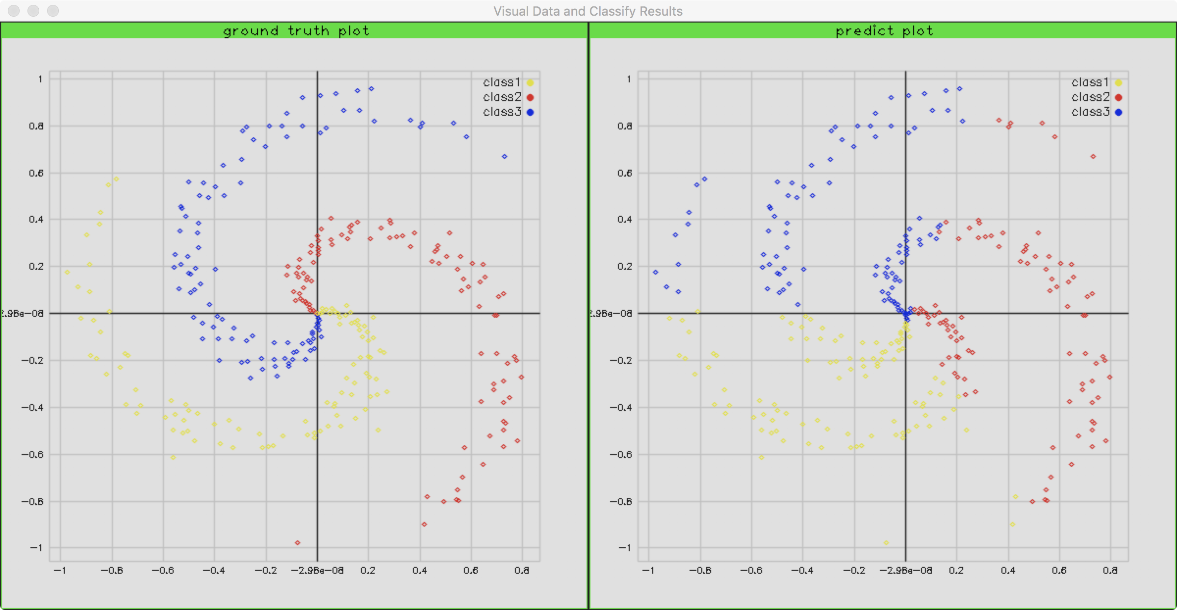
预测 最后,我们可以加载保存好的模型进行预测:
1 2 3 4 5 6 7 8 9 10 11 12 13 14 15 16 17 18 19 20 21 22 23 24 25 26 27 28 29 30 31 32 33 int * y_preds = new int [N * K];{ caffe2::Workspace workspace; caffe2::NetDef init_net, predict_net; caffe2::ModelUtil deploy_model (init_net, predict_net) ; deploy_model.Read (model_output); workspace.CreateBlob ("data" ); caffe2::Blob* input_blob = workspace.GetBlob ("data" ); caffe2::TensorCPU* input_tensor = input_blob->GetMutable <caffe2::TensorCPU>(); std::vector<int > dims = {N * K, D}; input_tensor->Resize (dims); float * input_data = input_tensor->mutable_data <float >(); std::copy (X, X + N * D * K, input_data); caffe2::Predictor predictor (init_net, predict_net, &workspace) ; caffe2::Predictor::TensorVector inputs, outputs; CAFFE_ENFORCE (predictor.run (inputs, &outputs)); const float * output_data = outputs[0 ]->data <float >(); for (int i = 0 ; i < N * K; ++i) { std::vector<float > probs (output_data + i * K, output_data + (i + 1 ) * K) ; std::vector<int > maxs = Argmax (probs, 1 ); y_preds[i] = maxs[0 ]; } }
当我们把结果绘制出来时,会发现长这个样子:
1
2
3
4
5
6
7
8
9
10
11
12
13
14
std::string Add (const std::string input_name, int in_size, int out_size) { predict.SetName ("FC" ); predict.AddInput (input_name); std::string layer = AddFcOps (input_name, "fc1" , in_size, 100 , true )->output (0 ); layer = AddFcOps (layer, "fc2" , 100 , out_size, false )->output (0 ); layer = predict.AddSoftmaxOp (layer, "prob" )->output (0 ); predict.AddOutput (layer); return layer; }
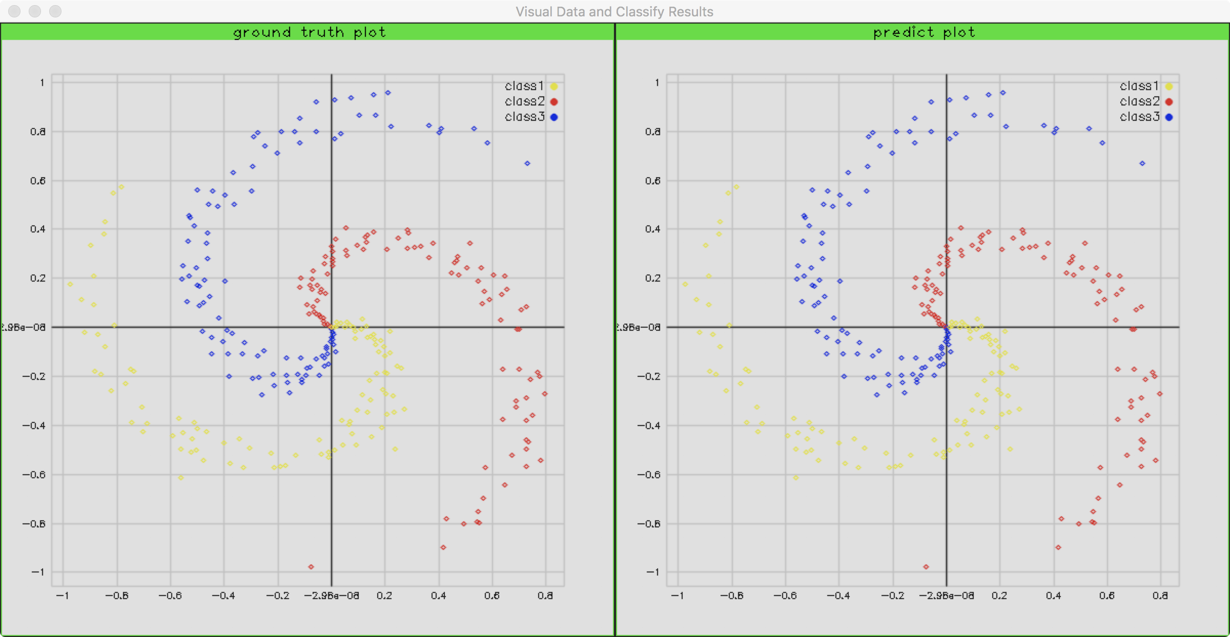
这里我们相当于添加了一个隐藏层,隐藏层的神经元数据为100。注意这里两个直连层之间多了一个ReLU激活,目的是为了增加神经网络对高维数据分布的拟合效果。当我们使用这个网络的时候,精度竟然达到了99.3%!下面是预测的结果和原来数据分布的对比: